Conformational Sampling

What conformational sampling is and why it is important

In computational chemistry, conformational sampling plays a crucial role in understanding the properties and reactivity of molecules. Conformational sampling refers to the exploration of different three-dimensional arrangements, or conformations, that a molecule can adopt. This spacial arrangement can greatly influence the properties of interest because of differences in the distances between atoms, in orbital interactions and in steric constraints, among other factors.

Molecules are exist in dynamic environments, constantly undergoing thermal motion and fluctuating between a range of conformations. What we mean by "conformation" is a local minimum in terms of all molecular coordinates, the bottom of a potential well on the potential energy surface (PES). In reality, molecules do not adopt strictly this conformation, but oscillates around this local minimum until it crosses over to another local minimum.

In the context of computational chemistry, we often use conformations (the minima) in order to study the properties of the molecule in its state of flux. However, determining the most energetically favorable or relevant conformations for a given molecule is a complex task due to the high dimensionality of the conformational space, namely $3N - 6$ dimensions (or $3N - 5$ for linear molecules). Conformational sampling methods aim to address this challenge by efficiently exploring this vast space and identifying all the significant local minima.

How conformations are found

Various algorithms and techniques have been developed to explore the conformational space effectively. These include systematic search methods, such as the systematic torsion angle sampling or grid-based techniques, as well as stochastic search methods, like Monte Carlo methods and molecular dynamics simulations. Each approach has its strengths and limitations, and the choice of method depends on the specific objectives and computational resources available.

One relatively recent solution to this problem has been developed and made freely available by the group of Stefan Grimme in a software called CREST. This approach makes extensive use of the extremely fast GFNn-xTB methods (available through the xtb package), which enable dynamics simulations for all the supported elements (hydrogen to radon). These simulations could be done using standard forcefields instead of GFNn-xTB, but this is very restrictive in terms of the supported molecules. Indeed, most forcefields have been developed with peptides and proteins in mind. Other molecules can be simulated using forcefields if proper parameters can be developed for these specific molecules. The GFNn-xTB methods thus provide a very convenient way to simulate the dynamics of almost any molecule. Moreover, the Grimme group have developed a forcefield method inspired from the GFNn-xTB methods and developed an automated parameterization procedure in order to keep the same generality. Among the three GFNn-xTB methods (n from 0 to 2), GFN2-xTB is the most accurate, and thus we will only consider this method out of the three here.

Conformational sampling is achieved by using molecular dynamics simulations to find new conformers. Starting from the initial conformation of the molecule, multiple other conformations will be explored throughout the simulations, purely through the random atomic movements within the molecule. With long enough simulations, all conformations will be visited by the molecule.

However, depending on the flexibility of the molecule and the conformational change barriers, the required simulation time might be unreasonable in these conditions. In order to accelerate the exploration of new conformations, an artificial potential is periodically added around the current configuration. This potential increases the potential energy of the geometries that have been explored and thus "lowers" the barriers to new conformations. This can be seen as pouring a bucket of sand in the potential well and reducing its depth. After this has been done enough times, the potential well will be very shallow and the molecule will exit it towards new conformations. This type of dynamics is called meta-dynamics and is extensively used in the CREST package. Meta-dynamics are discussed in more detail in S. Grimme, J. Chem. Theory Comput., 2019, 155, 2847-2862.

The full conformational sampling procedure is explained in details on the CREST documentation. In brief, meta-dynamics simulations are used to iteratively explore more and more possible conformations until no lower energy conformation is found. The structures that are found are reoptimized and filtered down to unique conformations. Normal molecular dynamics are launched starting from the most stable conformers in order to explore nearby conformations. Finally, the new orientations of parts of the molecule are applied to other conformers in order to generate a hybrid conformation, which is likely of similar energy as its parents. This is called "Genetic Z-matrix crossing", as it uses an approach related to genetic algorithms to combined conformations into new ones without relying on dynamics simulation.

The computational cost of conformational sampling

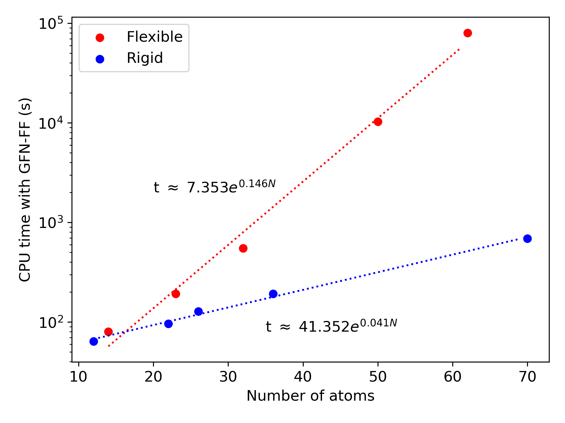
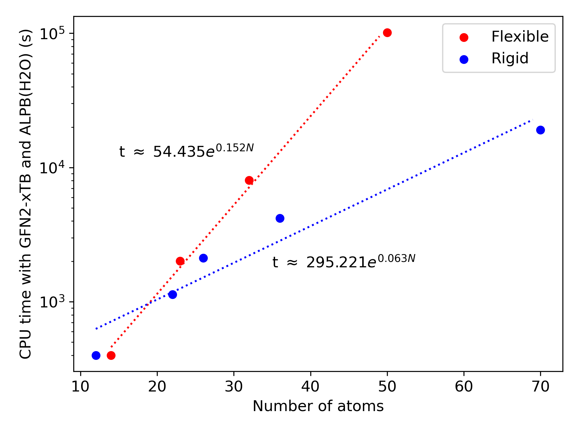
The time required to perform the conformational sampling increases rapidly with the number of atoms in the molecule and its flexibility. To give you an idea of the resources required for your molecules, we have benchmarked the conformational search of very flexible molecules (linear alkanes) and very rigid molecules (insaturated polycycles). The GFN2-xTB calculations also used the analytical linearized Poisson-Boltzmann (ALPB) implicit solvation model to represent a typical use case (see S. Ehlert, M. Stahn, S. Spicher, S. Grimme, J. Chem. Theory Comput., 2021, 17, 4250-4261). The calculations were performed using 8 vCPU cores on CalcUS Cloud. The time reported is the computing time used, which is 8 times greater than the real elapsed time.

Name	Number of atoms	CPU Time (GFN-FF)	CPU Time (GFN2-xTB/ALPB(H2O))	Number of conformers*
Butane	14	80	400	2
Heptane	23	192	2008	16-17
Decane	32	552	8040	33-48
Hexadecane	50	10304	101488	143-197
Eicosane	62	80264	-	999
Benzene	12	64	400	1
Biphenyl	22	96	1136	1-2
Pyrene	26	128	2120	1
Coronene	36	336	4200	1
Bicoronene	70	688	19112	1-2

*This number can vary greatly depending on the parameters used, notably the maximal relative energy and the threshold RMSD for unique conformers (see the text for more details).

While the conformational sampling of small molecules like butane and benzene required similar durations, the different quickly increases. In the extreme case, we can compare eicosane ($C_{20}H_{42}$), which took 22 CPU-hours with GFN-FF, to bicoronene ($C_{48}H_{22}$), which took under 12 CPU-minutes, despite having slightly more atoms.

The conformational sampling compute time grows exponentially with the number of atoms, and the flexibility of the molecules dictates how fast the time will grow. The two figures below illustrate the enormous difference between the rigid insaturated hydrocarbons in blue and the flexible alkane chains in red. The two series follow quite closely an exponential curve for molecules between 12 and 70 atoms. We can thus use the trendlines as guides to predict the minimal and maximal compute times to expect from a molecule with a given number of atoms. We can hardly predict exactly how much time the conformational sampling will take, but we can be confident that it will be between these two extremes.

How unique conformations are identified

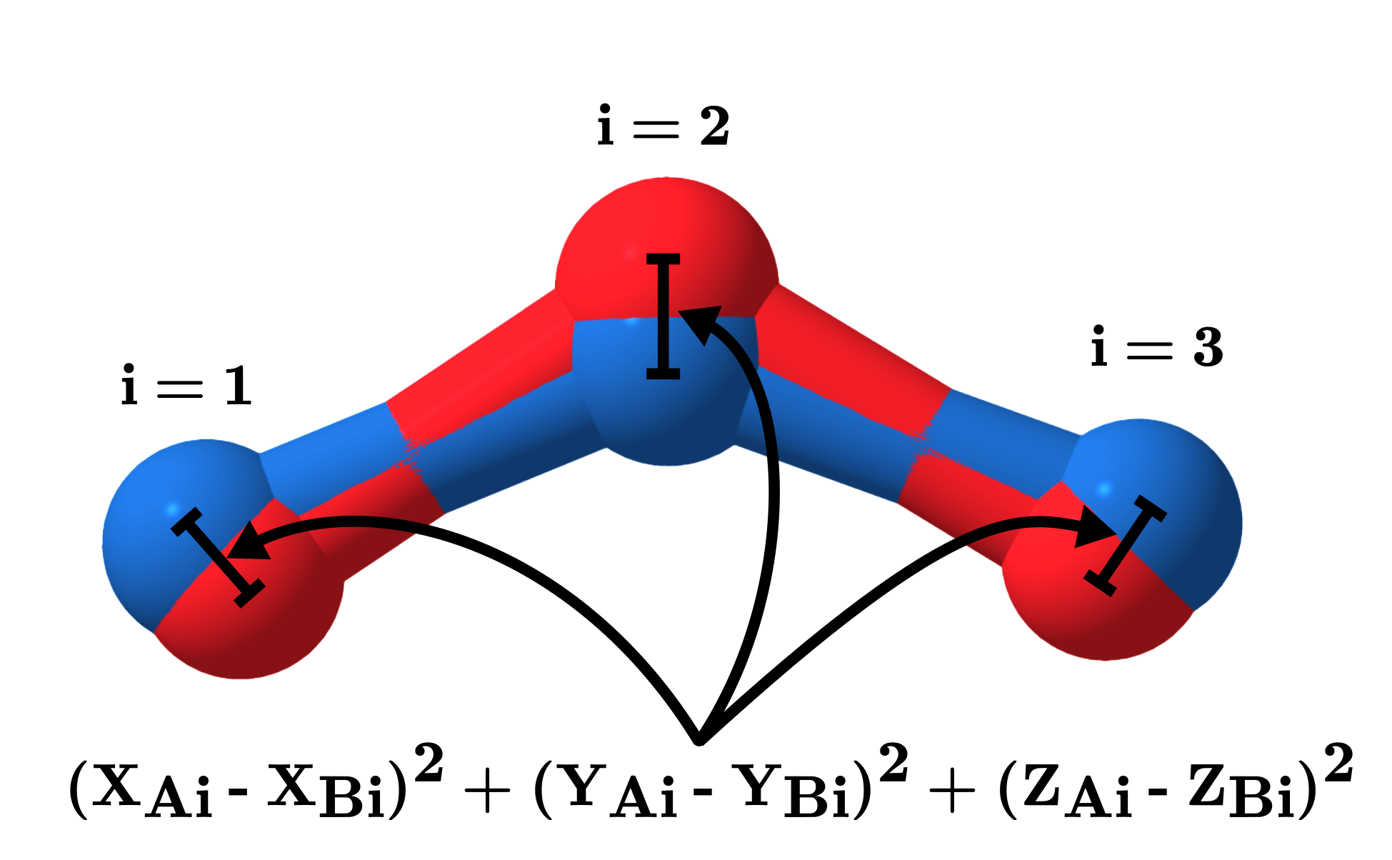
The conformational search process generates a large number of structures which may or may not correspond to known conformers. Even if two structures are visually indistinguishable to the human eye, its numerical representation (i.e., the 3D coordinates of the atoms) will not be identical. This is because structures remain chemically identical after translations or rotations, while the numerical representation is completely different. Moreover, tiny variations in the coordinates would make the coordinates different, while humans would classify them as essentially identical.

In order to compare structures mathematically more rigorously, we can use their root mean squared deviation (RMSD) as difference metric. In words, this criteria expresses the average magnitude of the deviation between the position of the atoms in one structure compared to the other. It is usually implicitly assumed that both structures have been aligned (through translations and rotations) in order to obtain the smallest RMSD possible. This means that two structures whose internal coordinates are identical will have a RMSD of 0 with respect to each other. If the structures have slightly different bond distances or different angles within the molecule, the RMSD will quantify to what extent the structures differ.

RMSD = $\sqrt{\frac{\sum_{i=1}^N \left((x_{Ai} - x_{Bi})^2 + (y_{Ai} - y_{Bi})^2 + (z_{Ai} - z_{Bi})^2\right)}{N}}$

Example: the structure of $NO_2$

Both structures were aligned in order to minimize the RMSD. Due to the different N-O bond distances and O-N-O angles, the atoms are slightly offset. In this case, the RMSD is 0.125 Å, which is quite small.

In the context of conformational sampling, we use a certain threshold RMSD above which two structures are considered to be different conformations. By default, the RMSD threshold of conformational searches on CalcUS Cloud is 2.0 Å, which is generally suitable for molecules with average flexibility and moderate size. However, if you wish to change this threshold, you can use the calculation specification --rthr NEWVALUE when launching the calculation. Additional available options are explained in the CalcUS documentation.

There are however some caveats with respect to the RMSD. It requires all the atoms to be distinguishable, meaning that we know with which atom in structure B we should compare each atom in structure A. While this is generally not a problem, it can cause duplicate conformers if there are equivalent atoms in the molecule. For example, a methyl group has three equivalent hydrogen atoms. If the methyl group rotates by 120 degrees, the structure is chemically identical, since there is still three hydrogen atoms at the same positions. However, the indices of these atoms are different, meaning that the RMSD will compare the positions of the "wrong" hydrogen atoms and will not be null. It is thus possible that these two structures will be considered to be two unique conformations, although this is chemically false.

General Recipe

1. Select your input structure on the launch page, either through the online sketcher or by uploading the structure in a suitable format.
2. Specify the molecule name, the solvent (if desired), the project and pick the xtb software. The calculation type should be "Conformational Search".
3. Decide on the best method to use. Refer to the table above to estimate the approximate CPU time required with each method. If your system contains transition metals or exotic valence, it would be wise to optimise the structure using GFN-FF to verify if its structure changes significantly. If it does, GFN-FF might not be suitable. If the computing time is reasonable, using GFN2-xTB is a safe choice.
4. If desired, add specifications.
5. Submit the calculation and wait for it to finish. Conformational searches do not start immediately like other xtb calculations, since they are executed on an entire virtual machine, which takes some time to start up.
6. Once the calculation is done, click on the calculation order to view the ensemble page. You will see a table with all the unique conformers ranked by energy.
7. Use the ensemble (or a subset of it) for further calculations (e.g., frequency calculation to calculate the free energy). The Boltzmann-weighted ensemble averages will be calculated for energetic properties (energy and free energy). These values are more representative of the true value of the molecule than any individual conformation, since they take into account all (unique) significant conformations.

Tips and guidelines

• The more polar the solvent, the more implicit solvation is important. Without implicit solvation, the molecule will tend to curl up in order to maximize intramolecular interactions. Implicit solvation adds the solvent-solute interactions which stabilize linear or "open" conformations. The increase in compute time caused by adding implicit solvation is pretty moderate.
• If you used GFN-FF, it is generally recommended to reoptimize all the structures using GFN2-xTB. You can launch the optimization for all structures by clicking on "Launch calculation on ensemble". You can also only consider the relevant conformers by holding the Control key and clicking on table entries, then click "Launch calculation on selected structure(s)". GFN2-xTB optimizations take generally only a few seconds per structure, which is much less than the conformational search itself.