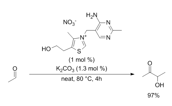
In this example, we are going to model the condensation of acetaldehyde into acetoin catalysed by vitamin B1 (ChemSusChem,
2014, 7(9), 2423–2426.)
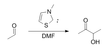
Firstly, we want to make the reaction more manageable by making some simplifications. The important part of vitamin B1 is the N-alkylated thiazole core; the rest will
participate in the reaction. We will thus model a simpler catalyst already in the N-Heterocyclic Carbene (NHC) form. Experimentally, vitamin B1 must be deprotonated to
achieve this form. However, computationally, we don't have to model this process. The neat conditions are also problematic, as only common solvents are parameterized in
computationnal chemistry software. We will thus use dimethylformamide (DMF) as solvent for the calculations, which is a good approximation of the substrate. The simplified
reaction we will study is thus:
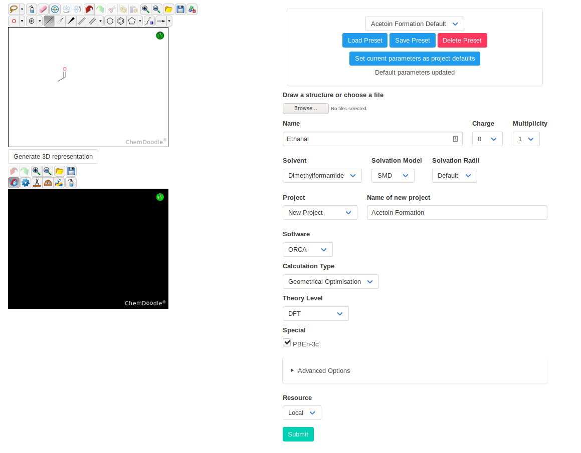
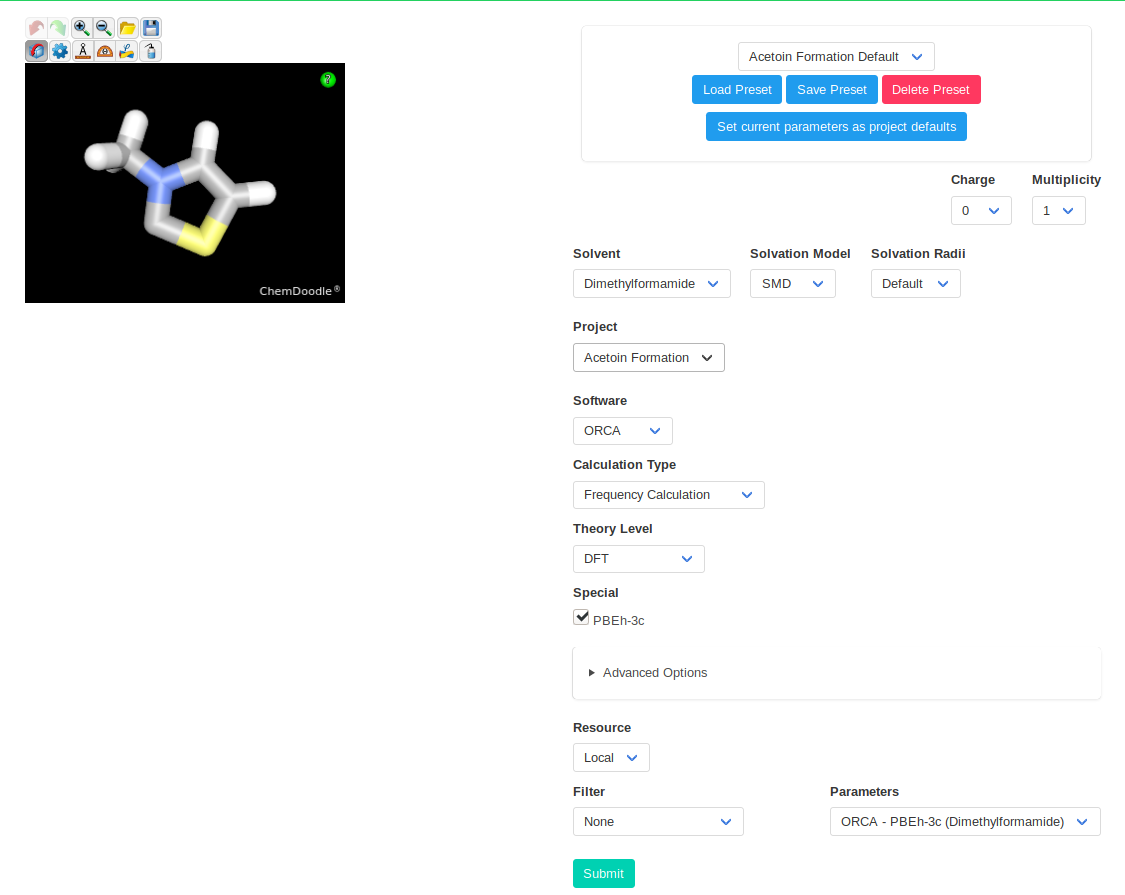
As computational method, we will use PBEh-3c with ORCA. This method is relatively fast while keeping most of the precision of "normal" DFT. It uses a minimized basis set
with three corrections and has been shown to have a good accuracy for thermodynamic values. SMD will be used as solvation model with DMF as solvent.
Initial Species
We will start by optimizing ethanal and creating the new project. Once we have chosen the right settings, you can save them as project default. They will be loaded any time
this project is selected.
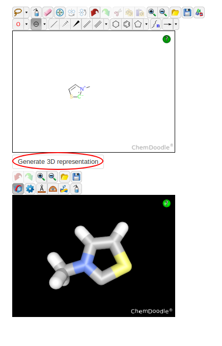
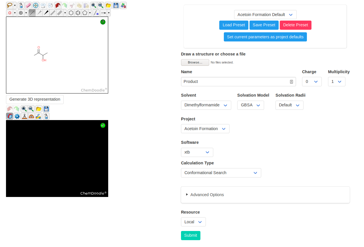
For the catalyst, the right input in the ChemDoodle sketcher is slightly trickier. You can verify that it yields the right structure by using the "Generate 3D
Representation" button.
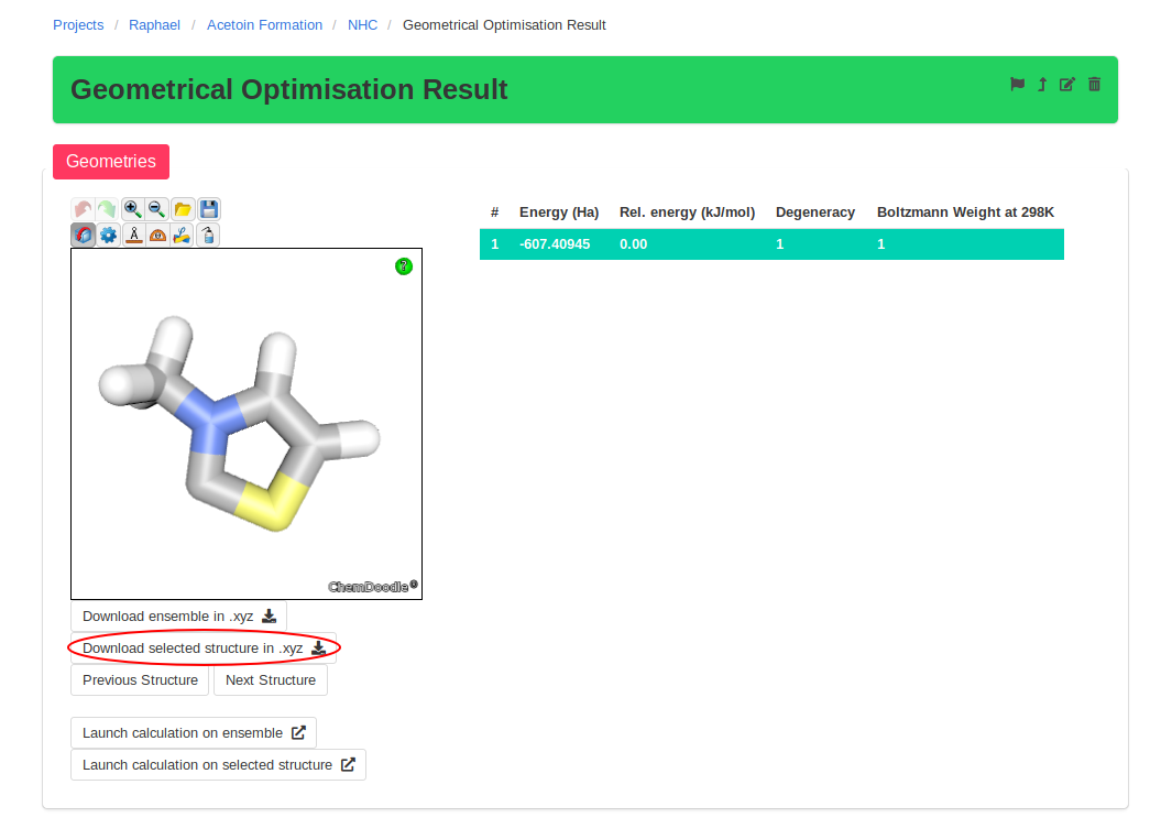
For every new equilibrium structure, you will want to perform a frequency calculation to obtain the thermochemical corrections. This can be done on an entire ensemble by
clicking on "Launch calculation on ensemble" on the ensemble page. Afterwards, it is a good idea to verify the vibrational frequencies obtained. For equilibrium structures,
they should all be positive, while transition states should have only one negative frequency.
To simplify the final analysis, CalcUS uses a flagging system. Each ensemble has a flag icon which can be turned on (light grey) or off (black). This mechanism will allow
to sort out the final structures from all the calculations that lead to them. This will become especially useful in the following sections.
NHC Addition
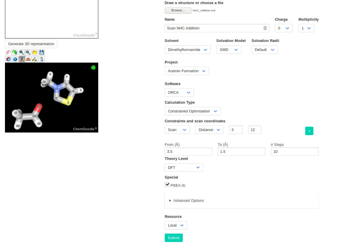
The next step is finding the transition state (TS) of addition of the NHC catalyst to the substrate. The sketcher does not support multiple species, but you can download
the optimized structure of the catalyst and modify it.
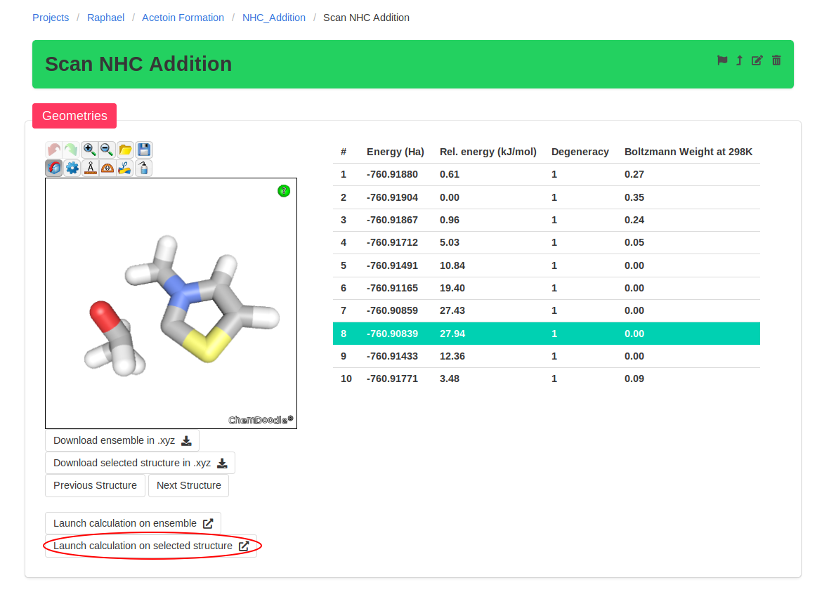
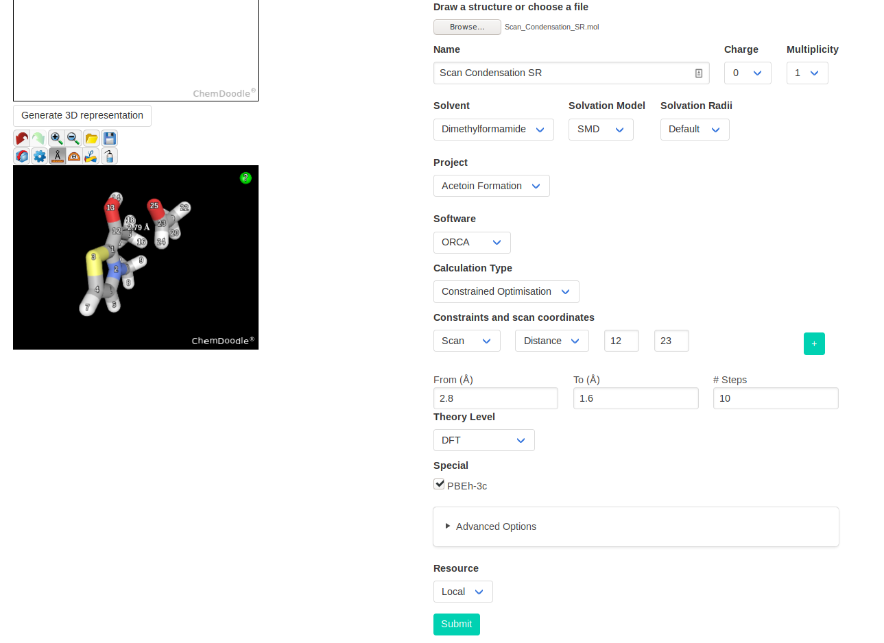
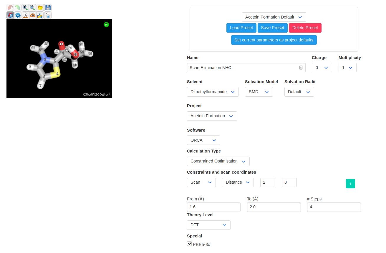
You can then launch a constrained optimisation on your initial structure. We will perform a relaxed scan of the distance between the nucleophilic NHC carbon and the
electrophilic carbonyl carbon. With this scan, we find the approximate path to the addition product; the point highest in energy of the scan should be relatively close to
the TS.
As can be seen below, we obtain an approximate TS where the carbon-carbon bond is half-formed and the carbonyl has started to pyramidalize. We will use this structure as
guess for a TS optimisation, which we can launch using the button "Launch calculation on selected structure". Simply use the same parameters as before and change the
calculation type to "TS Optimisation".
A frequency calculation will confirm that we have obtained the desired structure. You should observe only one negative frequency, and the animation should show oscillation
of the bond in formation.
We will also perform a geometrical optimisation on a structure past the TS to obtain the addition product.
Breslow Intermediates and Condensation
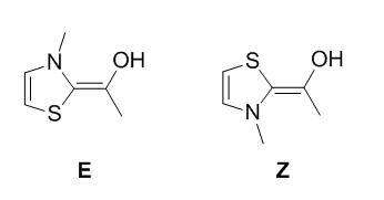
After the addition, a proton transfer will yield either the Z or E Breslow intermediate. The mechanism of the proton transfer is uncertain and likely involves multiple
species. We will not try to find the transition state, as this could be quite difficult.
As before, we will download the XYZ structure of both Breslow intermediates and add ethanal. Note however that both intermediates can perform the addition on either side of
the ethanal, yielding different relative stereochemistries. We will thus have to find 4 transition states. Instead of performing 4 relaxed scans, we will perform only one.
After finding a first transition state, we will modify it to obtain the desired relative stereochemistries. For example, if we find the addition TS of the Z Breslow
intermediate with anti stereochemistry, we can have a very good guess of the addition TS for the E Intermediate by turning the aromatic core by 180 degrees. To obtain the
syn stereochemistry, we can put a methyl group instead of the hydrogen of the ethanal and delete the other methyl. Make sure to reoptimize the transition state afterwards!
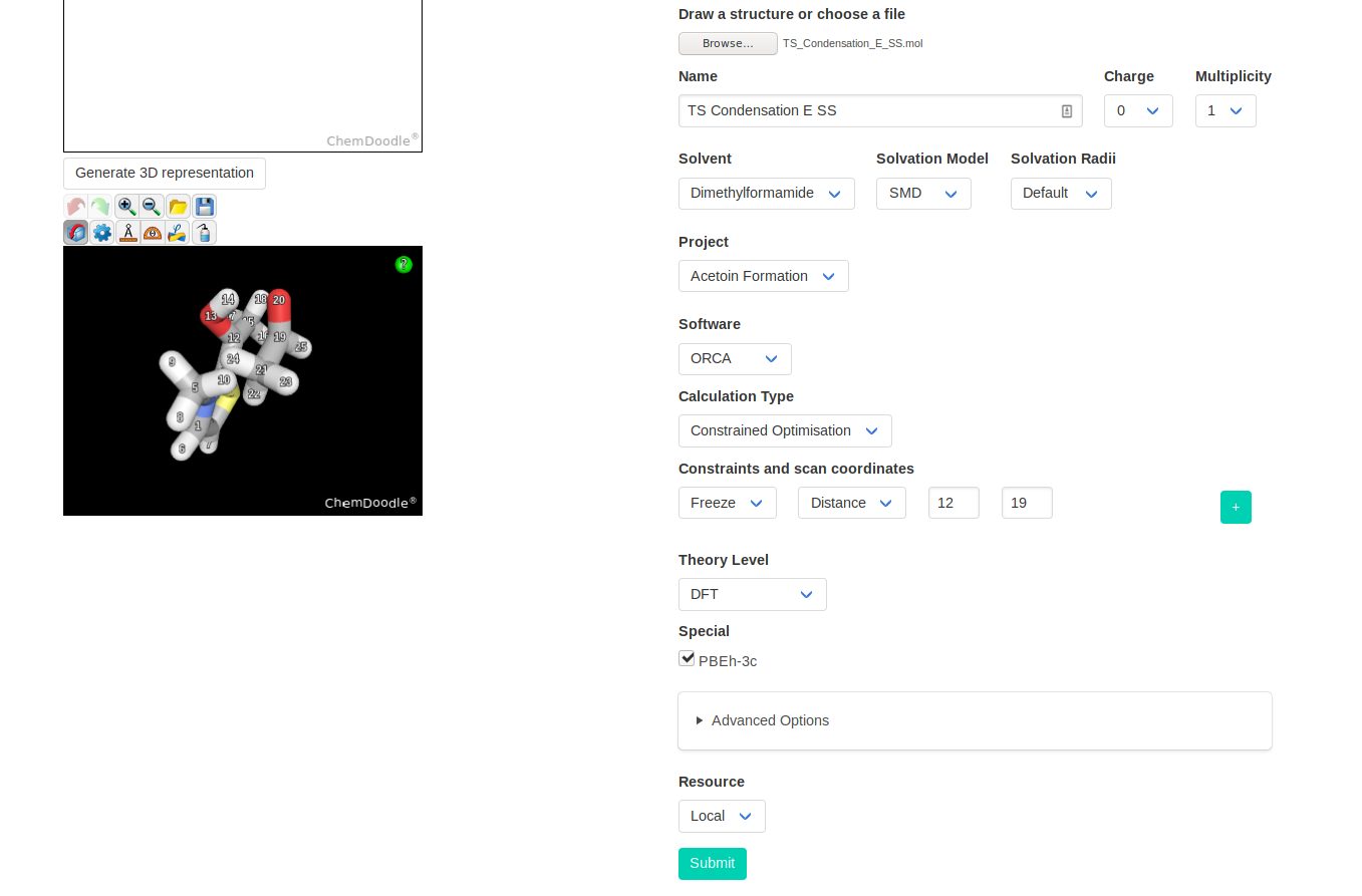
If there is important steric clashes in the TS guess, we can preoptimize the structure with a frozen carbon-carbon bond. This will allow the structure to relax, except for
the bond in formation. Although it adds one extra step, it can help the software to identify the real reaction coordinate by relaxing all others to minima.
We will also optimise the condensation products, starting either from the last step of the relaxed scan or from scratch. With PBEh-3c, the proton transfer between the two
oxygens can occur spontaneously during the geometrical optimisation. As such, we will consider the two forms in rapid equilibrium and use the most stable form obtained.
Performing a conformational search would be a good idea, but GFN2-xTB appears to generate unexpected new bonds in this case.
Catalyst Regeneration and Final Product
For both anti and syn products, we just have to find the transition state of elimination/regeneration of the NHC catalyst. This is most easily done by stretching the
relevant carbon-carbon bond through a relaxed scan until it breaks. The point highest in energy should be a good TS guess. We will perform a TS optimisation on that
structure for both scans, followed by a frequency calculation to confirm and obtain the thermochemical corrections.
Finally, we need to model the final product. As it is quite flexible, we will sample its conformers with a conformational search (using the software xtb). This calculation
uses GFN2-xTB as computational method, and not our PBEh-3c. This means that we cannot directly use the results in our study. However, we can use the structures obtained in
this way as starting points for calculations with PBEh-3c. This allows us to take advantage of the fast conformational sampling of xtb while having final results with
PBEh-3c (or any other desired method).
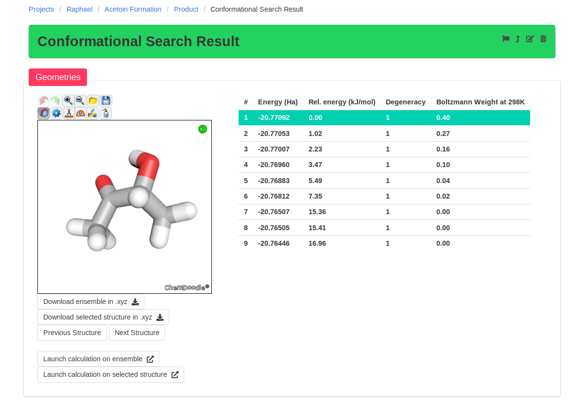
After the conformational search, we see that the last three conformers are much higher in energy and do not contribute significantly to the Boltzmann average. These
conformers don't have to be reoptimized.
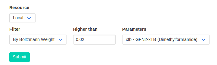
CalcUS offers the convenient option to filter them on the submission page. When launching a calculation on an ensemble, the "Filter" option will appear at the bottom of the
options. Here, we will reoptimize any conformer which contributes more than 2% to the total Boltzmann average.
This will create a new ensemble with only the remaining conformers. We will then perform frequency calculations on this new ensemble using PBEh-3c.
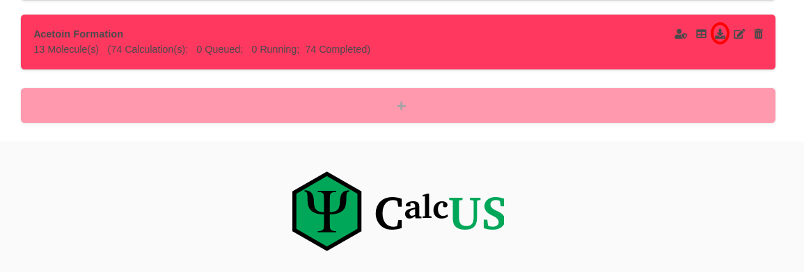
Analysis
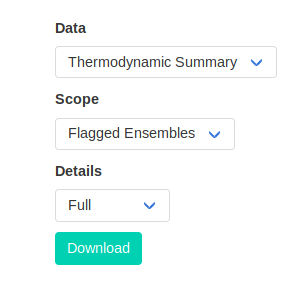
To obtain the summary of the thermodynamic properties for all the project, we can click on the download icon.
We will download only the flagged ensemble, as we do not need the energies of all the scans, conformational searches, etc. By manually flagging the ensembles we need along
the way, we eliminate the headache of sorting through all the calculations we have performed.
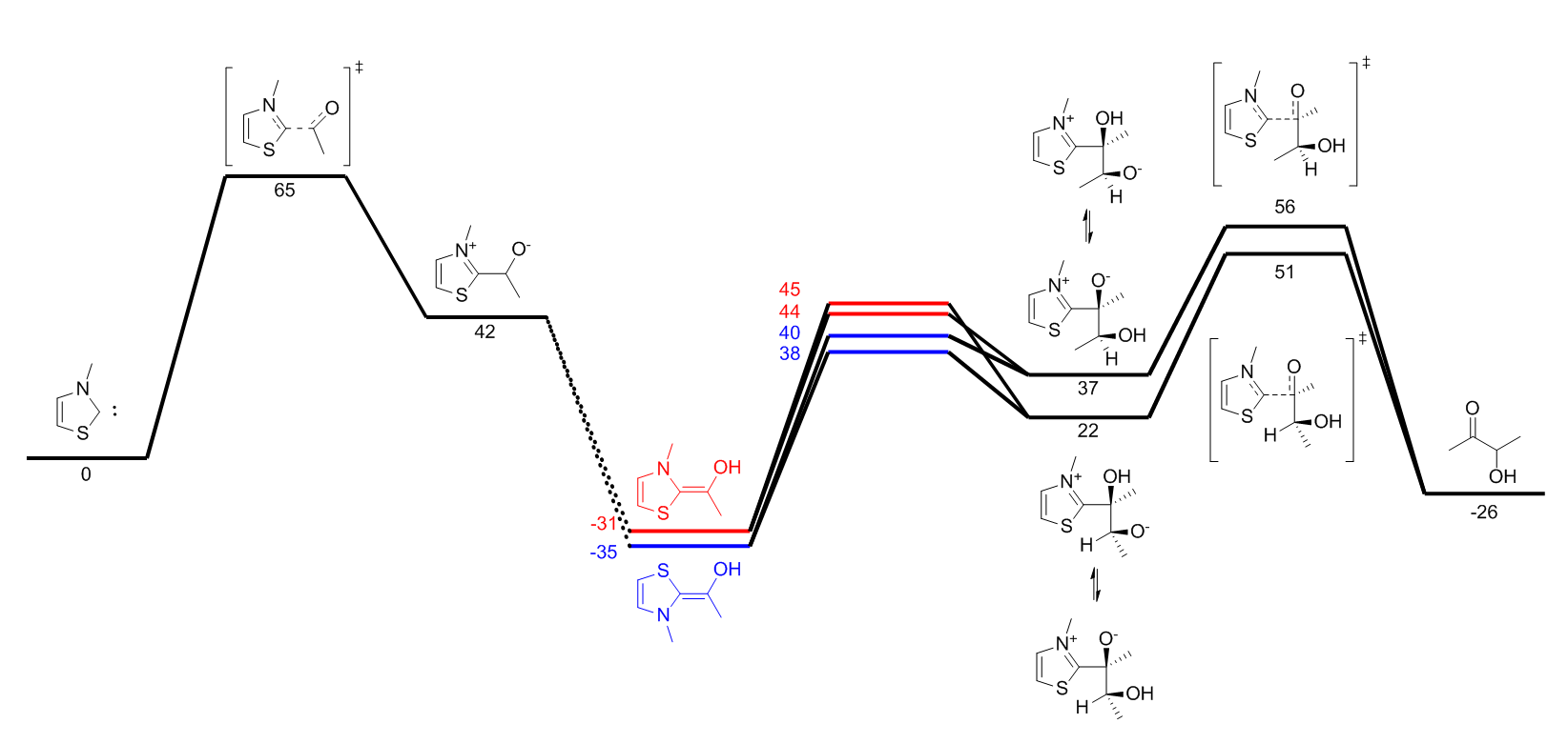
This will create a CSV file which can be opened in any spreadsheet software. We will use these values to compute the relative free energies of every relevant point in the
reaction with respect to the starting product. For each intermediate, take its free energy and substract from it the free energy of every specie that went into its
formation. You should obtain an energy profile which looks like the following.
Version d4c33ab
By using our website, you consent to our use of cookies. We use cookies to keep you logged in, see if you're new here and provide a better user experience. See the details
 Firstly, we want to make the reaction more manageable by making some simplifications. The important part of vitamin B1 is the N-alkylated thiazole core; the rest will
participate in the reaction. We will thus model a simpler catalyst already in the N-Heterocyclic Carbene (NHC) form. Experimentally, vitamin B1 must be deprotonated to
achieve this form. However, computationally, we don't have to model this process. The neat conditions are also problematic, as only common solvents are parameterized in
computationnal chemistry software. We will thus use dimethylformamide (DMF) as solvent for the calculations, which is a good approximation of the substrate. The simplified
reaction we will study is thus:
Firstly, we want to make the reaction more manageable by making some simplifications. The important part of vitamin B1 is the N-alkylated thiazole core; the rest will
participate in the reaction. We will thus model a simpler catalyst already in the N-Heterocyclic Carbene (NHC) form. Experimentally, vitamin B1 must be deprotonated to
achieve this form. However, computationally, we don't have to model this process. The neat conditions are also problematic, as only common solvents are parameterized in
computationnal chemistry software. We will thus use dimethylformamide (DMF) as solvent for the calculations, which is a good approximation of the substrate. The simplified
reaction we will study is thus:
 As computational method, we will use PBEh-3c with ORCA. This method is relatively fast while keeping most of the precision of "normal" DFT. It uses a minimized basis set
with three corrections and has been shown to have a good accuracy for thermodynamic values. SMD will be used as solvation model with DMF as solvent.
As computational method, we will use PBEh-3c with ORCA. This method is relatively fast while keeping most of the precision of "normal" DFT. It uses a minimized basis set
with three corrections and has been shown to have a good accuracy for thermodynamic values. SMD will be used as solvation model with DMF as solvent.
 For the catalyst, the right input in the ChemDoodle sketcher is slightly trickier. You can verify that it yields the right structure by using the "Generate 3D
Representation" button.
For the catalyst, the right input in the ChemDoodle sketcher is slightly trickier. You can verify that it yields the right structure by using the "Generate 3D
Representation" button.
 For every new equilibrium structure, you will want to perform a frequency calculation to obtain the thermochemical corrections. This can be done on an entire ensemble by
clicking on "Launch calculation on ensemble" on the ensemble page. Afterwards, it is a good idea to verify the vibrational frequencies obtained. For equilibrium structures,
they should all be positive, while transition states should have only one negative frequency.
For every new equilibrium structure, you will want to perform a frequency calculation to obtain the thermochemical corrections. This can be done on an entire ensemble by
clicking on "Launch calculation on ensemble" on the ensemble page. Afterwards, it is a good idea to verify the vibrational frequencies obtained. For equilibrium structures,
they should all be positive, while transition states should have only one negative frequency.
 To simplify the final analysis, CalcUS uses a flagging system. Each ensemble has a flag icon which can be turned on (light grey) or off (black). This mechanism will allow
to sort out the final structures from all the calculations that lead to them. This will become especially useful in the following sections.
To simplify the final analysis, CalcUS uses a flagging system. Each ensemble has a flag icon which can be turned on (light grey) or off (black). This mechanism will allow
to sort out the final structures from all the calculations that lead to them. This will become especially useful in the following sections.

 You can then launch a constrained optimisation on your initial structure. We will perform a relaxed scan of the distance between the nucleophilic NHC carbon and the
electrophilic carbonyl carbon. With this scan, we find the approximate path to the addition product; the point highest in energy of the scan should be relatively close to
the TS.
You can then launch a constrained optimisation on your initial structure. We will perform a relaxed scan of the distance between the nucleophilic NHC carbon and the
electrophilic carbonyl carbon. With this scan, we find the approximate path to the addition product; the point highest in energy of the scan should be relatively close to
the TS.
 As can be seen below, we obtain an approximate TS where the carbon-carbon bond is half-formed and the carbonyl has started to pyramidalize. We will use this structure as
guess for a TS optimisation, which we can launch using the button "Launch calculation on selected structure". Simply use the same parameters as before and change the
calculation type to "TS Optimisation".
As can be seen below, we obtain an approximate TS where the carbon-carbon bond is half-formed and the carbonyl has started to pyramidalize. We will use this structure as
guess for a TS optimisation, which we can launch using the button "Launch calculation on selected structure". Simply use the same parameters as before and change the
calculation type to "TS Optimisation".
 A frequency calculation will confirm that we have obtained the desired structure. You should observe only one negative frequency, and the animation should show oscillation
of the bond in formation.
A frequency calculation will confirm that we have obtained the desired structure. You should observe only one negative frequency, and the animation should show oscillation
of the bond in formation.
 As before, we will download the XYZ structure of both Breslow intermediates and add ethanal. Note however that both intermediates can perform the addition on either side of
the ethanal, yielding different relative stereochemistries. We will thus have to find 4 transition states. Instead of performing 4 relaxed scans, we will perform only one.
After finding a first transition state, we will modify it to obtain the desired relative stereochemistries. For example, if we find the addition TS of the Z Breslow
intermediate with anti stereochemistry, we can have a very good guess of the addition TS for the E Intermediate by turning the aromatic core by 180 degrees. To obtain the
syn stereochemistry, we can put a methyl group instead of the hydrogen of the ethanal and delete the other methyl. Make sure to reoptimize the transition state afterwards!
As before, we will download the XYZ structure of both Breslow intermediates and add ethanal. Note however that both intermediates can perform the addition on either side of
the ethanal, yielding different relative stereochemistries. We will thus have to find 4 transition states. Instead of performing 4 relaxed scans, we will perform only one.
After finding a first transition state, we will modify it to obtain the desired relative stereochemistries. For example, if we find the addition TS of the Z Breslow
intermediate with anti stereochemistry, we can have a very good guess of the addition TS for the E Intermediate by turning the aromatic core by 180 degrees. To obtain the
syn stereochemistry, we can put a methyl group instead of the hydrogen of the ethanal and delete the other methyl. Make sure to reoptimize the transition state afterwards!
 If there is important steric clashes in the TS guess, we can preoptimize the structure with a frozen carbon-carbon bond. This will allow the structure to relax, except for
the bond in formation. Although it adds one extra step, it can help the software to identify the real reaction coordinate by relaxing all others to minima.
If there is important steric clashes in the TS guess, we can preoptimize the structure with a frozen carbon-carbon bond. This will allow the structure to relax, except for
the bond in formation. Although it adds one extra step, it can help the software to identify the real reaction coordinate by relaxing all others to minima.
 We will also optimise the condensation products, starting either from the last step of the relaxed scan or from scratch. With PBEh-3c, the proton transfer between the two
oxygens can occur spontaneously during the geometrical optimisation. As such, we will consider the two forms in rapid equilibrium and use the most stable form obtained.
Performing a conformational search would be a good idea, but GFN2-xTB appears to generate unexpected new bonds in this case.
We will also optimise the condensation products, starting either from the last step of the relaxed scan or from scratch. With PBEh-3c, the proton transfer between the two
oxygens can occur spontaneously during the geometrical optimisation. As such, we will consider the two forms in rapid equilibrium and use the most stable form obtained.
Performing a conformational search would be a good idea, but GFN2-xTB appears to generate unexpected new bonds in this case.
 Finally, we need to model the final product. As it is quite flexible, we will sample its conformers with a conformational search (using the software xtb). This calculation
uses GFN2-xTB as computational method, and not our PBEh-3c. This means that we cannot directly use the results in our study. However, we can use the structures obtained in
this way as starting points for calculations with PBEh-3c. This allows us to take advantage of the fast conformational sampling of xtb while having final results with
PBEh-3c (or any other desired method).
Finally, we need to model the final product. As it is quite flexible, we will sample its conformers with a conformational search (using the software xtb). This calculation
uses GFN2-xTB as computational method, and not our PBEh-3c. This means that we cannot directly use the results in our study. However, we can use the structures obtained in
this way as starting points for calculations with PBEh-3c. This allows us to take advantage of the fast conformational sampling of xtb while having final results with
PBEh-3c (or any other desired method).
 After the conformational search, we see that the last three conformers are much higher in energy and do not contribute significantly to the Boltzmann average. These
conformers don't have to be reoptimized.
After the conformational search, we see that the last three conformers are much higher in energy and do not contribute significantly to the Boltzmann average. These
conformers don't have to be reoptimized.
 CalcUS offers the convenient option to filter them on the submission page. When launching a calculation on an ensemble, the "Filter" option will appear at the bottom of the
options. Here, we will reoptimize any conformer which contributes more than 2% to the total Boltzmann average.
CalcUS offers the convenient option to filter them on the submission page. When launching a calculation on an ensemble, the "Filter" option will appear at the bottom of the
options. Here, we will reoptimize any conformer which contributes more than 2% to the total Boltzmann average.
 This will create a new ensemble with only the remaining conformers. We will then perform frequency calculations on this new ensemble using PBEh-3c.
 We will download only the flagged ensemble, as we do not need the energies of all the scans, conformational searches, etc. By manually flagging the ensembles we need along
the way, we eliminate the headache of sorting through all the calculations we have performed.
We will download only the flagged ensemble, as we do not need the energies of all the scans, conformational searches, etc. By manually flagging the ensembles we need along
the way, we eliminate the headache of sorting through all the calculations we have performed.
 This will create a CSV file which can be opened in any spreadsheet software. We will use these values to compute the relative free energies of every relevant point in the
reaction with respect to the starting product. For each intermediate, take its free energy and substract from it the free energy of every specie that went into its
formation. You should obtain an energy profile which looks like the following.
This will create a CSV file which can be opened in any spreadsheet software. We will use these values to compute the relative free energies of every relevant point in the
reaction with respect to the starting product. For each intermediate, take its free energy and substract from it the free energy of every specie that went into its
formation. You should obtain an energy profile which looks like the following.