Stationary Points on the Potential Energy Surface (PES)

Where the potential energy surface comes from

A given molecule is determined by the types (elements) and positions of its nuclei in certain electronic quantum state. The energy of this electronic quantum state can be evaluated by solving the fundamental equation of quantum mechanics, the Schrödinger equation. In particular, we will look at the time-independent Schrödinger equation:

$\hat H \Psi(r, R) = E \Psi(r, R)$

where $\hat H$ is the Hamiltonian operator, which contains the physical equations to calculate the energy, roughly speaking; $\Psi(r, R)$ is the full quantum mechanical wavefunction of the molecule, which depends on the position of its electrons ($r$) and of its nuclei ($R$), which are 3D vectors. While there are often more than one electron and nucleus, we use a single symbol to represent each set of positions for the sake of simplicity. However, you should known that:

$r = (\vec r_1, \vec r_2, ..., \vec r_i) = ((r_{1\; x}, r_{1\; y}, r_{q \; z}), ...)$.

This equation is what is called an eigenvalue equation. This particular type of equation features the same variable on both sides of the equality ($\Psi(r, R)$, in this case). The Hamiltonian operator applies mathematical operations to $\Psi(r, R)$, so we cannot simply cancel them out like in more conventional algebra. The equation is then a relationship between the unknown function $\Psi(r, R)$ and itself. Solving this equation for more than one particle is a formidable task. Luckily there is a good approximation that allows its simplification considerably. It is the Born-Oppenheimer approximation of separating the nuclear and electronic motion. The fact is that the electrons are much smaller than even the smallest nucleus, the proton, and move much faster than the nuclei in a molecule. The electrons can be viewed as an electron cloud that follows (relaxes) almost instantly with any change of the nuclei positions.

Mathematically, this means that the approximation states that $\Psi(r, R) \approx \Psi(r)\Phi(R)$, where $\Psi(r)$ is now the wavefunction of only the electrons and $\Phi(R)$ is the wavefunction of only the nuclei. If we chose the positions of the nuclei $R$, then $\Phi(R)$ is fixed and easy to compute. The challenge lies in the evaluation of the molecular electronic energy, since the positions of the electrons $r$ are unknown and cannot be considered to be fixed.

For completeness, the equation we need to solve is $\hat H \Psi(r) = E_{el \; R} \Psi(r)$, where $E_{el \; R}$ is the electronic energy when the nuclei have position $R$. We can compute the total energy of the molecule by adding the electrostatic repulsion between (necessarily positively charged) nuclei $E_{nuc \; R}$. Thus:

$E_{tot \; R} = E_{el \; R} + E_{nuc \; R}$

What the potential energy surface is

The previous section was only concerned with one single set of nuclear positions $R$. However, these positions can take an infinity of values, although only a small portion of them is useful to compute. For each set of nuclear positions, we can compute a corresponding electronic energy. The potential energy surface (PES) is the collection of electronic energies associated to all nuclear positions, which considered to be fixed within the Born-Oppenheimer approximation. We call it a surface, since it represents the smooth function of the electronic energy (dependent variable, denoted simply $E$) for each set of nuclear positions (independent variables).

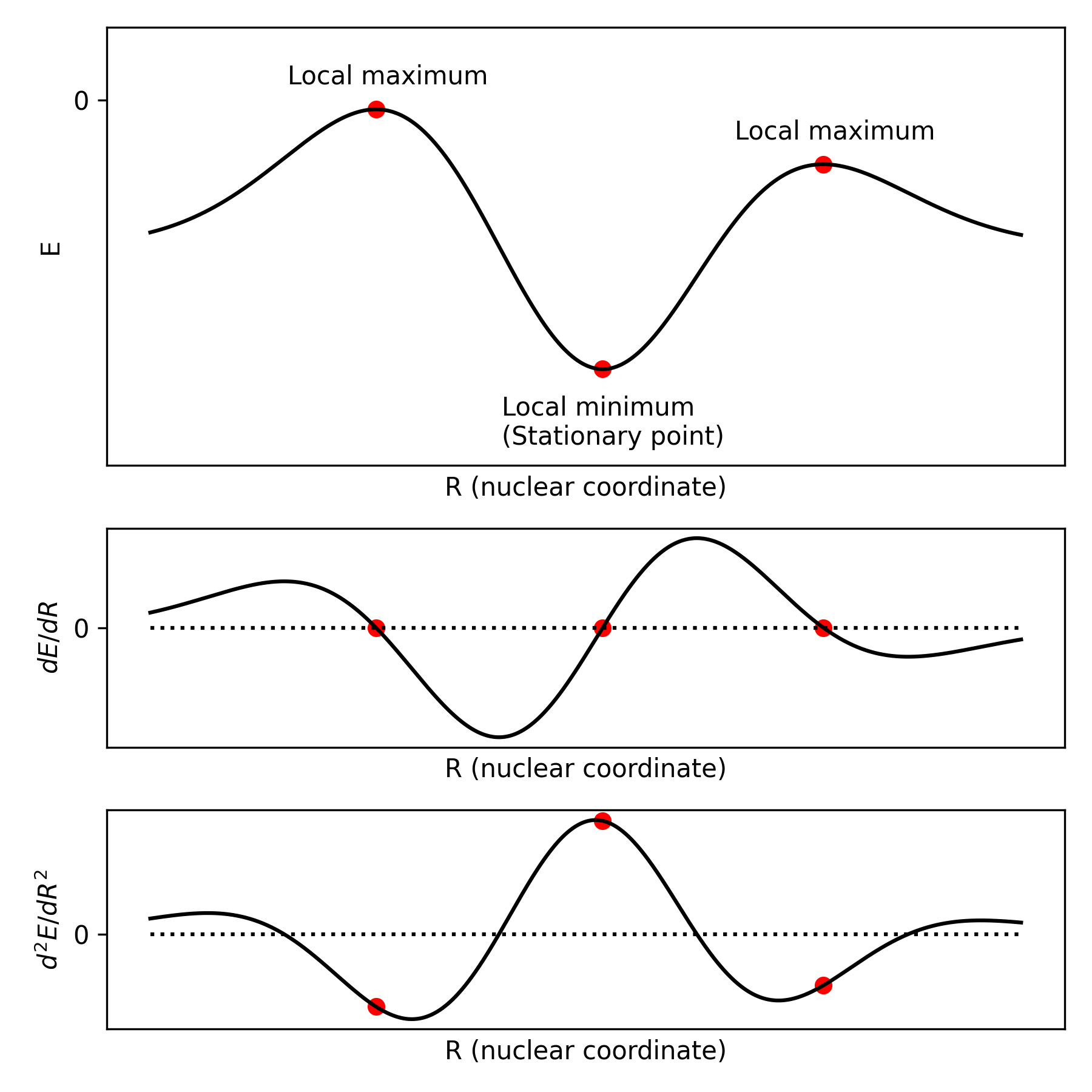
In quantum chemistry, we are mostly interested in two types of points on this surface: minima, corresponding to the most stable structure of the molecule, and saddle points, which correspond to transition states. There can be multiple local minima and saddle points on the potential energy surface. Minima can correspond to conformers of the same molecule, reaction intermediates, or stable products of some reactions. Each saddle point will correspond to the transition between two minima.

In this lesson, we will look at the minima (also denoted "stationary points" or "equilibrium geometries"), as they are simpler to understand. For a single-variable function like $E(R)$, we know from calculus that the first derivative $dE/dR$ is going to be zero at each minima. Moreover, the second derivative $d^2E/dR^2$ will be positive, since the potential energy surface curves upwards.

Simple 1 dimensional potential energy surface

Internal coordinates

As mentioned before, the nuclear (cartesian) coordinates $R$ represent the positions of all nuclei in the system. In its most intuitive form, this means the 3D positions of each atom in space, thus yielding $3N$ coordinates for $N$ atoms (however they may be bonded). While valid, this representation has some shortcomings in computational chemistry. Firstly, we may consider how a translation of the entire system may influence these coordinates. Since there is no "true origin", every properties will be exactly the same regardless of where the system starts in space. However, a translation of the entire system will change the 3D coordinates of all atoms, as we consider them to be moved by a certain quantity in a certain direction. It thus appears that some coordinate changes don't influence the results at all, while others clearly do. The same thing is true when considering rotations of the entire system.

Secondly, these cartesian coordinates can be needlessly complex to handle computationally. Let's consider the dihydrogen molecule. To define its structure, we need 6 cartesian coordinates, as shown below. Then, if we want to optimize the geometry, we will need to calculate the gradient of the energy with respect to these coordinates (i.e., the previously mentioned $dE/dR$). The gradient will need to represent how the energy changes when each of these six coordinates changes.

The structure of $H_2$ in cartesian coordinates

However, we know that most of that information is useless, since there is only one meaningful coordinate: the bond length. Regardless of how you move the atoms, the only thing that will influence the properties is how the bond length changed. We can thus can only compute the gradient of the energy with respect to the bond length and have the same information. Very simply, this means that we have only one value to compute instead of six. (As always, the reality is a bit more complex, but this example illustrates the important point.)

More generally, structures will be converted from cartesian coordinates to internal coordinates by calculation packages. These internal coordinates eliminates the "external coordinates" related to translation and rotation. The result is $3N - 6$ internal coordinates for $N$ atoms, except for linear systems, where we obtain $3N - 5$ internal coordinates. This exception is because the rotation around the axis of linear systems does not exist, as it does not change the position of any atom in cartesian space. For dihydrogen, a linear molecule, we obtain $3*2 - 5 = 1$ internal coordinate, namely the bond length.

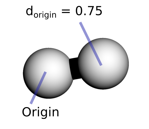
The structure of $H_2$ in internal coordinates

The first atom is defined as the origin, the reference position of the system. The second atom is defined by its distance from the first atom. In larger systems, the third atom will be defined by its distance from the second atom as well as the angle formed by these three atoms, and the fourth atom will be defined by a distance, an angle as well as a dihedral angle formed by these four atoms. Additional atoms will also require three coordinates to be unambiguously defined.

Example: visualization of one internal coordinate of butane

This example is discussed in more detail in the lesson on conformational sampling

While molecules have many internal coordinates, we can selectively plot a single one for given values. The animation below shows the potential energy curve associated with variations in the C-C-C-C dihedral angle of butane.

In this case, the minima are States A and C, which correspond to possible conformations of the same molecule. States B and D are maxima as well as saddle points (although the other coordinates are not displayed) which connect each stable conformation.

Speed

Manual Animation

Geometrical optimizations

When modelling molecules, stationary points are generally what we're looking for. A geometrical optimization is the type of calculation that allows us to obtain stationary points. The calculation starts with an initial structure that you create or obtain from someone (for example, in a scientific publication). The energy gradient is computed for that structure and used to determine what to do next. If the gradient is small enough, then the structure is a minimum for all intents and purposes and the calculation is done. Otherwise, the gradient is used to guess which structure is very likely lower in energy. Visually, the gradient is a vector on the potential energy surface that points towards the steepest increase in energy. To obtain structures lower in energy, the atoms just have to be moved in the exact opposite direction, towards the steepest descent in energy. The atoms are displaced by a small distance before the energy gradient is calculated again. This is because the gradient we calculated is only valid for the point at which we calculated it; as we move atoms, the gradient changes. To find the minimum, we need to iteratively calculate a gradient and move atoms by small measures.

In practice, many algorithms exist to carry out this procedure and they vary on how they approach this iterative procedure. For example, some algorithms calculate or estimate the second derivative of the energy in order to guess more accurately how far to move atoms at each step. The goal of more complex algorithms is to reduce the number of steps needed to obtain the minimum, and thus reduce the computing time. Fortunately, as users of existing quantum chemistry packages, we rarely need to worry about the details of these algorithms and the procedures are carried out automatically.

General Recipe

Go to the launch page and select an input structure, either through the online sketcher or by uploading the structure in a suitable format.
Specify the molecule name, the solvent (if desired), the project and pick the xtb software. The calculation type should be "Geometrical Optimization".
Submit the calculation and wait for it to finish. For structures under 100 atoms, this should take only seconds.
Once the calculation is done, click on the calculation order to view the ensemble page. You will see the optimized structure as well as its energy. By clicking the ruler icon above the structure, you can measure distances between atoms. The two icons on the right allow you to measure angles and dihedral angles respectively.
To view the optimization steps, go back to the calculation order page, find the order corresponding to the same calculation, then click on the list icon at the top right (the three lines). Then click on the calculation id, which is a yellow button. You will see a 3D structure alongside a curve which gradually decreases to almost zero (if the optimization was successful). You can go through the different optimization steps by using the scroll bar under the structure or by clicking on points in the graph. If your initial structure is close to optimal, it might be difficult to see any change between the frames; try with a larger molecule with multiple substituents and sidechains.

Tips and guidelines

In almost all cases, properties have to be calculated on optimized geometries. After optimizing a geometry, you can launch subsequent property calculations on it to obtain meaningful results. Otherwise, you will obtain the properties of the specific unoptimized geometries you used, which will not be very representative of the real molecular structure.
GFN2-xTB generally yields good enough geometries. Except if you require high accuracy results (for a scientific publication, for example), the geometries optimized with the GFN2-xTB method are often good enough. Systems with exotic functional groups, transition metals or other less common elements might be problematic, but this has to be determined for each specific case. Geometries obtained with DFT functionals and a good basis set are almost always very good.